Introduction

I have finally finished undergrad and would like to make a blog post about what I have been working on these past ~6 months. The tile of our thesis is:

ClaudesLens: Uncertainty Quantification in Computer Vision Models

Which you can read here

However, before I dive into the project and what we actually did, let me tell you what we wanted to do.

BayesLens

Originally, we wanted to create “Uncertainty-Aware Attention Mechanisms”. What we specifically had in mind was to create a transformer model that used Bayesian Neural Networks (BNNs), and even more ambitiously, apply this to self-driving cars.

Needless to say, this was a bit too ambitious for a BSc thesis, so we had to scale down our project a bit. We didn’t have the prerequisite knowledge or the compute to do such a task within that time frame and with other courses.

So about ~1/3 into the project, when our supervisor wanted us to explore the entropy of predictions and got really excited about our results, we got ClaudesLens.

ClaudesLens

From the results using entropy as a measure of uncertainty, we decided to focus on this instead. I’ll go into more detail and motivate how this approach works, but believe that this is a very natural way to quantify uncertainty.

I plan to explain this project from the ground up, from first principles so to say, so let’s start what lies at the heart of this project: Neural Networks.

Neural Networks

There are many ways to explain neural networks, in this post I will use a mathematical approach which will let us view the entire network as a single function.

The Neuron

At the core of a neural network lies the neuron, which is inspired by the biological neuron.

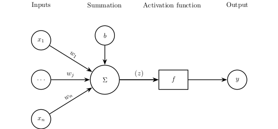
Each neuron takes in one or more scalars, $x_j$, as input and outputs a single scalar, $y$. Each input, $x_j$, is scaled by an associated weight denoted as $w_j$. The neuron also has a special input called the bias, $b$.

The neuron has two stages it goes through, summation and activation.

Figure 1: A single neuron with n inputs and one output, showcasing the summation and activation components.

The summation stage is where the neuron calculates the weighted sum of the inputs and the bias: $$ z = \sum_{j=1}^{n} w_j x_j + b $$

The activation function, denoted as $f$, calculates the neuron’s output $y = f(z)$ based on the weighted summation. Activation functions introduce non-linearity, enabling neural networks to approximate complex, non-linear functions.

The Network

Lets build upon what we now have learned and see how we can extend this.

We can represent the inputs of a neuron as a vector, $$ \mathbf{x} = \left[x_1, x_2, \ldots, x_n\right], $$

where each element corresponds to an input to the neuron.

Similarly, we can represent the associated weights as a vector, $$ \mathbf{w} = \left[w_1, w_2, \ldots, w_n\right], $$

with this the summation can be simplified to a dot product, $$ z = \mathbf{w} \cdot \mathbf{x} + b. $$

But only using one neuron will only get us so far, if we instead have multiple neurons and try to mimic the structure of the brain, we can get something more powerful.

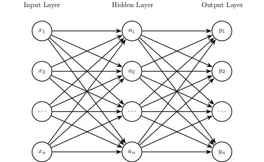
A layer is a collection of neurons, stacked on top of each other. Very often when we are referring to a layer, are we referring to a fully connected layer, where each neuron in the layer is connected to all the neurons in the previous layer.

In the case of a network, we can now talk about the input layer and the output layer.

Figure 2: A simple neural network with one hidden layer.

As we see in the picture, we now have multiple neurons with numerous inter-neuron connections, along with multiple outputs.

The matrix-vector equation, $$ \mathbf{a} = \mathbf{W_1} \mathbf{x} + \mathbf{b_1} = [a_1, a_2, \ldots, a_m], $$

yields each output of each neuron in the hidden layer.

$\mathbf{W_1}$ is the weight matrix with rows $\mathbf{w_i} = [w_{i, 1}, w_{i, 2}, \ldots, w_{i, n}]$ corresponding to the weights of the $i$-th neuron in the hidden layer. The bias values are represented by $\mathbf{b_1} = [b_1, b_2, \ldots, b_m]$.

In the case of several layers, we work with multiple weight matrices and bias vectors, which we index as $\mathbf{W_j}$ and $\mathbf{b_j}$, respectively.

So, given an input $\mathbf{x}$, the output of the hidden layer (i.e figure 2) is given by, $$ \mathbf{a} = f.(\mathbf{W_1} \mathbf{x} + \mathbf{b_1}), $$

where the dot indicates that the activation function $f$ is applied element-wise.

So the final output is therefore, $$ \mathbf{y} = f.(\mathbf{W_2} \mathbf{a} + \mathbf{b_2}). $$

This is the basic structure of a neural network, for the sake of brevity I will not go into more detail about the training process, but I will mention that these weights and biases are learned through an optimization process called backpropagation.

There are a ton of resources to understand these concepts, even we tried to explain these concepts in our thesis.

Computer Vision

Now that we have a basic understanding of neural networks, we can move on to computer vision.

Computer vision is a field of computer science that focuses on replicating parts of the complexity of the human vision system and enabling computers to identify and process objects in images and videos in the same way that humans do.

The most important thing that we will cover here is how we represent images, which is crucial for understanding how we can apply neural networks to images.

Images

Images are represented as a grid of pixels, where each pixel needs to be represented in a numerical way.

For most images, we represent each pixel as a 3-dimensional vector, where each element corresponds to the intensity of the color channels red, green, and blue (RGB). This is called a channel.

So, a single pixel in an image is represented as a vector, therefore a whole image can be represented as a 3-dimensional tensor.

Remember this.

Entropy-based Uncertainty Quantification Framework

I’ll try to keep this quite short and sweet, again, in our paper we go into more detail, but from what we have seen, we can view a neural network as a function.

In our case, our model, since we’re dealing with classification, will spit out a probablity vector, and we always choose the class with the highest probability, ergo, $$ \hat{y} = \arg\max(\mathcal{F}(\mathbf{x}, \mathbf{W})), $$

where $\mathcal{F}$ is our trained neural network, $\mathbf{x}$ is our input, and $\mathbf{W}$ are the trained weights of the network.

But this is deterministic, there is no uncertainty here, so how can we quantify this?

We make it stochastic.

By adding noise to the function, random noise, it makes the function stochastic. If we do this multiple times, we can get a distribution of outputs, and from this distribution, we can calculate the entropy.

Entropy and Uncertainty

Now, when we are talking about entropy, we are talking about the information kind of entropy. Thanks to the great work of Claude Shannon, we have a way to quantify the uncertainty of a random variable.

The entropy of a random variable $X$ is defined as, $$ H(X) = -\sum_{x \in \chi} p(x) \log p(x), $$

where $p(x) = P(X = x)$.

Entropy in Neural Networks

So, if we have a neural network that outputs a probability distribution, we can calculate the entropy of this distribution. The entropy of a distribution is a measure of the uncertainty of the distribution, the higher the entropy, the more uncertain we are about the output. So, by adding noise to the function, we can calculate the entropy of the distribution of outputs, and this can give us a measure of the uncertainty of the model!

Conclusion

This is a very brief overview of what we did in our thesis, and I hope that I have motivated why we did what we did. I thought it was a very challenging but fun project, and I learned a lot from it.

Read the paper as well, we basically died writing it.